Week 5: Working with Tabular Data in Python with Pandas¶

This week, you will learn how to work with tabular data in Python.

Pandas is a an open source library providing high-performance, easy-to-use data structures and data analysis tools. Pandas is particularly suited to the analysis of tabular data, i.e. data that can can go into a table. In other words, if you can imagine the data in an Excel spreadsheet, then Pandas is the tool for the job.

A recent analysis of questions from Stack Overflow showed that python is the fastest growing and most widely used programming language in the world (in developed countries).

A follow-up analysis showed that this growth is driven by the data science packages such as numpy, matplotlib, and especially pandas.

The exponential growth of pandas is due to the fact that it just works. It saves you time and helps you do science more efficiently and effictively.

Pandas capabilities (from the Pandas website):¶

• A fast and efficient DataFrame object for data manipulation with integrated indexing;
• Tools for reading and writing data between in-memory data structures and different formats: CSV and text files, Microsoft Excel, SQL databases, and the fast HDF5 format;
• Intelligent data alignment and integrated handling of missing data: gain automatic label-based alignment in computations and easily manipulate messy data into an orderly form;
• Flexible reshaping and pivoting of data sets;
• Intelligent label-based slicing, fancy indexing, and subsetting of large data sets;
• Columns can be inserted and deleted from data structures for size mutability;
• Aggregating or transforming data with a powerful group by engine allowing split-apply-combine operations on data sets;
• High performance merging and joining of data sets;
• Hierarchical axis indexing provides an intuitive way of working with high-dimensional data in a lower-dimensional data structure;
• Time series-functionality: date range generation and frequency conversion, moving window statistics, moving window linear regressions, date shifting and lagging. Even create domain-specific time offsets and join time series without losing data;
• Highly optimized for performance, with critical code paths written in Cython or C.
• Python with pandas is in use in a wide variety of academic and commercial domains, including Finance, Neuroscience, Economics, Statistics, Advertising, Web Analytics, and more.

Let's start by importing pandas library.

In [1]:

import pandas as pd
import numpy as np

import pandas as pd import numpy as np

1. Basic Pandas¶

1.1 Basic data structures in Pandas:¶

Pandas provides two types of classes for handling data:

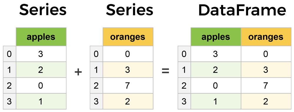
1. Series: a one-dimensional labeled array holding data of any type.
2. DataFrame: a two-dimensional data structure that holds data like a two-dimension array or a table with rows and columns.

You can think of Pandas Dataframe as an Excel spreadsheet, and Series as one column of the the spreadsheet. Multiple series can be combined as a DataFrame.

In [4]:

from IPython.display import Image
Image(url='https://storage.googleapis.com/lds-media/images/series-and-dataframe.width-1200.png')

from IPython.display import Image Image(url='https://storage.googleapis.com/lds-media/images/series-and-dataframe.width-1200.png')

Out[4]:

1.2 Pandas Series¶

Creating a Series by passing a list of values.

In [5]:

s = pd.Series([1, 3, 5, np.nan, 6, 8])

s = pd.Series([1, 3, 5, np.nan, 6, 8])

In [7]:

s

s

Out[7]:

0    1.0
1    3.0
2    5.0
3    NaN
4    6.0
5    8.0
dtype: float64

By default, Pandas creates a default RangeIndex starting from 0.

Creating a Series by passing values and indices.

In [9]:

s = pd.Series([1, 3, 5, np.nan, 6, 8], index = ['A','B','C','D','E','F'])
s

s = pd.Series([1, 3, 5, np.nan, 6, 8], index = ['A','B','C','D','E','F']) s

Out[9]:

A    1.0
B    3.0
C    5.0
D    NaN
E    6.0
F    8.0
dtype: float64

Pandas has plotting functions that can easily visualize the data.

In [11]:

s.plot(kind = 'bar')

s.plot(kind = 'bar')

Out[11]:

<Axes: >

Arithmetic operations and most numpy function can be applied to Series.

An important point is that the Series keep their index during such operations.

In [12]:

np.sqrt(s)

np.sqrt(s)

Out[12]:

A    1.000000
B    1.732051
C    2.236068
D         NaN
E    2.449490
F    2.828427
dtype: float64

We can also access the underlying index object if we need to:

In [13]:

s.index

s.index

Out[13]:

Index(['A', 'B', 'C', 'D', 'E', 'F'], dtype='object')

Exercise 1: Create a Pandas series with values ranging from 0 to 6, and label the index as the day of week, starting from 'Sunday' to 'Saturday'.¶

1.3 Indexing¶

We can get values back out using the index via the .loc attribute

In [14]:

s.loc['A']

s.loc['A']

Out[14]:

1.0

Or by raw position using .iloc:

In [15]:

s.iloc[0]

s.iloc[0]

Out[15]:

1.0

We can pass a list or array to loc to get multiple rows back:

In [21]:

s.loc[['A','C']]

s.loc[['A','C']]

Out[21]:

A    1.0
C    5.0
dtype: float64

We can also use the slice notation:

In [20]:

s.loc['A':'C']

s.loc['A':'C']

Out[20]:

A    1.0
C    5.0
dtype: float64

Exercise 2: Print out the last two elements of Series s (hint: using slice notation and iloc).¶

In [ ]:

1.4 Pandas data structure: DataFrame¶

A more useful Pandas data structure is the DataFrame. A DataFrame is basically a bunch of series that share the same index. It's a lot like a table in a spreadsheet.

Below we create a DataFrame.

In [61]:

# Data: AQI levels and temperature in different cities
data = {
    "AQI": [55, 75, 60, 80, np.NaN],
    "Temperature": [68, 75, 64, 80, 85]
}

# Creating the DataFrame
df = pd.DataFrame(data, index = ["New York", "Los Angeles", "Chicago", "Houston", "Phoenix"])

# Data: AQI levels and temperature in different cities data = { "AQI": [55, 75, 60, 80, np.NaN], "Temperature": [68, 75, 64, 80, 85] } # Creating the DataFrame df = pd.DataFrame(data, index = ["New York", "Los Angeles", "Chicago", "Houston", "Phoenix"])

In [62]:

df

df

Out[62]:

	AQI	Temperature
New York	55.0	68
Los Angeles	75.0	75
Chicago	60.0	64
Houston	80.0	80
Phoenix	NaN	85

In [63]:

# You can set the style of the table
df.style.highlight_max()

# You can set the style of the table df.style.highlight_max()

Out[63]:

	AQI	Temperature
New York	55.000000	68
Los Angeles	75.000000	75
Chicago	60.000000	64
Houston	80.000000	80
Phoenix	nan	85

You may notice that Pandas handles missing data very elegantly, keeping track of it through all calculations.

1.5 Index with Pandas DataFrame:¶

We can get a single column as a Series using python's getitem syntax on the DataFrame object.

In [64]:

df['AQI']

df['AQI']

Out[64]:

New York       55.0
Los Angeles    75.0
Chicago        60.0
Houston        80.0
Phoenix         NaN
Name: AQI, dtype: float64

...or using attribute syntax.

In [65]:

df.AQI

df.AQI

Out[65]:

New York       55.0
Los Angeles    75.0
Chicago        60.0
Houston        80.0
Phoenix         NaN
Name: AQI, dtype: float64

If you want to get a specific row, use .loc

In [66]:

df.loc['New York']

df.loc['New York']

Out[66]:

AQI            55.0
Temperature    68.0
Name: New York, dtype: float64

In [67]:

df.iloc[2]

df.iloc[2]

Out[67]:

AQI            60.0
Temperature    64.0
Name: Chicago, dtype: float64

But we can also specify the column and row we want to access:

In [68]:

df.loc['New York','AQI']

df.loc['New York','AQI']

Out[68]:

55.0

Exercise 3: Print out the temperature of Chicago and Los Angeles.¶

In [ ]:

1.6 Basic statistics with Pandas:¶

In [28]:

df.min()

df.min()

Out[28]:

AQI            55.0
Temperature    64.0
dtype: float64

In [30]:

df.idxmax()

df.idxmax()

Out[30]:

AQI            Houston
Temperature    Phoenix
dtype: object

In [31]:

df.mean()

df.mean()

Out[31]:

AQI            67.5
Temperature    74.4
dtype: float64

In [32]:

df.count()

df.count()

Out[32]:

AQI            4
Temperature    5
dtype: int64

In [33]:

df.std()

df.std()

Out[33]:

AQI            11.902381
Temperature     8.561542
dtype: float64

In [34]:

# describe function can print out the descriptive statistics easily!
df.describe()

# describe function can print out the descriptive statistics easily! df.describe()

Out[34]:

	AQI	Temperature
count	4.000000	5.000000
mean	67.500000	74.400000
std	11.902381	8.561542
min	55.000000	64.000000
25%	58.750000	68.000000
50%	67.500000	75.000000
75%	76.250000	80.000000
max	80.000000	85.000000

Exercise 4: Print out the city with minimum temperature.¶

In [ ]:

1.7 Modifying Pandas DataFrame¶

Add new row:

In [69]:

df.loc['New Brunswick'] = [64, 75]

df.loc['New Brunswick'] = [64, 75]

In [70]:

df

df

Out[70]:

	AQI	Temperature
New York	55.0	68
Los Angeles	75.0	75
Chicago	60.0	64
Houston	80.0	80
Phoenix	NaN	85
New Brunswick	64.0	75

Add new column:

In [71]:

df['Cloudy'] = [True, False, True, False, False, True]

df['Cloudy'] = [True, False, True, False, False, True]

In [72]:

df

df

Out[72]:

	AQI	Temperature	Cloudy
New York	55.0	68	True
Los Angeles	75.0	75	False
Chicago	60.0	64	True
Houston	80.0	80	False
Phoenix	NaN	85	False
New Brunswick	64.0	75	True

In [73]:

data = {
    "Latitude": [40.7128, 34.0522, 41.8781, 29.7604, 33.4484],
    "Longitude": [-74.0060, -118.2437, -87.6298, -95.3698, -112.0740]
}

df_loc = pd.DataFrame(data, index = ["New York", "Los Angeles", "Chicago", "Houston", "Phoenix"])

data = { "Latitude": [40.7128, 34.0522, 41.8781, 29.7604, 33.4484], "Longitude": [-74.0060, -118.2437, -87.6298, -95.3698, -112.0740] } df_loc = pd.DataFrame(data, index = ["New York", "Los Angeles", "Chicago", "Houston", "Phoenix"])

In [74]:

df_loc

df_loc

Out[74]:

	Latitude	Longitude
New York	40.7128	-74.0060
Los Angeles	34.0522	-118.2437
Chicago	41.8781	-87.6298
Houston	29.7604	-95.3698
Phoenix	33.4484	-112.0740

Combine df and df_loc:

In [75]:

df_join = df.join(df_loc)

df_join = df.join(df_loc)

In [77]:

df_join

df_join

Out[77]:

	AQI	Temperature	Cloudy	Latitude	Longitude
New York	55.0	68	True	40.7128	-74.0060
Los Angeles	75.0	75	False	34.0522	-118.2437
Chicago	60.0	64	True	41.8781	-87.6298
Houston	80.0	80	False	29.7604	-95.3698
Phoenix	NaN	85	False	33.4484	-112.0740
New Brunswick	64.0	75	True	NaN	NaN

In [79]:

df_join = df.join(df_loc, how = 'right')
df_join

df_join = df.join(df_loc, how = 'right') df_join

Out[79]:

	AQI	Temperature	Cloudy	Latitude	Longitude
New York	55.0	68	True	40.7128	-74.0060
Los Angeles	75.0	75	False	34.0522	-118.2437
Chicago	60.0	64	True	41.8781	-87.6298
Houston	80.0	80	False	29.7604	-95.3698
Phoenix	NaN	85	False	33.4484	-112.0740

Using concat to append new rows:

In [80]:

df_append = pd.concat([df,df_loc])

df_append = pd.concat([df,df_loc])

In [81]:

df_append

df_append

Out[81]:

	AQI	Temperature	Cloudy	Latitude	Longitude
New York	55.0	68.0	True	NaN	NaN
Los Angeles	75.0	75.0	False	NaN	NaN
Chicago	60.0	64.0	True	NaN	NaN
Houston	80.0	80.0	False	NaN	NaN
Phoenix	NaN	85.0	False	NaN	NaN
New Brunswick	64.0	75.0	True	NaN	NaN
New York	NaN	NaN	NaN	40.7128	-74.0060
Los Angeles	NaN	NaN	NaN	34.0522	-118.2437
Chicago	NaN	NaN	NaN	41.8781	-87.6298
Houston	NaN	NaN	NaN	29.7604	-95.3698
Phoenix	NaN	NaN	NaN	33.4484	-112.0740

2. Advanced Pandas¶

2.1 Importing tabular data in pandas¶

In Pandas, the most commonly used function to import tabular data is read_csv function

As you can see, pd.read_csv() has quite a few parameters. Don't be overwhelmed – most of these are optional arguments that allow you to specify exactly how your data file is structured and which part(s) you want to import. In particular, the sep parameter allows the user to specify the type of delimiter used in the file. The default is a comma, but you can actually pass other common delimiters (such as sep='\t', which is a tab) to import other delimited files. The only required argument is a string specifying the filepath of your file.

In [ ]:

pd.read_csv?

pd.read_csv?

Download wildfire data Spatial_Database_Big_Wildfires_US_all.csv from Canvas, and upload the data to your current working directory.

In [84]:

df = pd.read_csv('Spatial_Database_Big_Wildfires_US_all.csv')
df.head()

df = pd.read_csv('Spatial_Database_Big_Wildfires_US_all.csv') df.head()

Out[84]:

	FOD_ID	FPA_ID	SOURCE_SYSTEM_TYPE	SOURCE_SYSTEM	NWCG_REPORTING_UNIT_ID	NWCG_REPORTING_UNIT_NAME	FIRE_CODE	FIRE_NAME	MTBS_FIRE_NAME	COMPLEX_NAME	...	CONT_DOY	FIRE_SIZE	FIRE_SIZE_CLASS	LATITUDE	LONGITUDE	OWNER_DESCR	STATE	COUNTY	FIPS_CODE	FIPS_NAME
0	17	FS-1418878	FED	FS-FIRESTAT	USCAENF	Eldorado National Forest	NaN	POWER	POWER	NaN	...	295.0	16823.0	G	38.523333	-120.211667	USFS	CA	5	6005.0	Amador County
1	18	FS-1418881	FED	FS-FIRESTAT	USCAENF	Eldorado National Forest	BHA3	FREDS	FREDS	NaN	...	291.0	7700.0	G	38.780000	-120.260000	USFS	CA	17	6017.0	El Dorado County
2	40	FS-1418920	FED	FS-FIRESTAT	USNCNCF	National Forests in North Carolina	BKC8	AUSTIN CREEK	NaN	NaN	...	44.0	125.0	D	36.001667	-81.590000	MISSING/NOT SPECIFIED	NC	27	37027.0	Caldwell County
3	119	FS-1419153	FED	FS-FIRESTAT	USNENBF	Nebraska National Forest	BEW8	THOMPSON BUTTE	NaN	NaN	...	198.0	119.0	D	43.899167	-102.954722	USFS	SD	103	46103.0	Pennington County
4	120	FS-1419156	FED	FS-FIRESTAT	USNENBF	Nebraska National Forest	BEW8	CHARLES DRAW	NaN	NaN	...	197.0	119.0	D	43.892778	-102.948056	USFS	SD	103	46103.0	Pennington County

5 rows × 28 columns

2.2 Groupby methods¶

groupby is an amazingly powerful function in pandas, but it is also complicated to use and understand. The point of this section is to make you feel confident in using groupby.

In [85]:

df.columns

df.columns

Out[85]:

Index(['FOD_ID', 'FPA_ID', 'SOURCE_SYSTEM_TYPE', 'SOURCE_SYSTEM',
       'NWCG_REPORTING_UNIT_ID', 'NWCG_REPORTING_UNIT_NAME', 'FIRE_CODE',
       'FIRE_NAME', 'MTBS_FIRE_NAME', 'COMPLEX_NAME', 'FIRE_YEAR',
       'DISCOVERY_DATE', 'DISCOVERY_DOY', 'DISCOVERY_TIME',
       'NWCG_CAUSE_CLASSIFICATION', 'NWCG_GENERAL_CAUSE',
       'NWCG_CAUSE_AGE_CATEGORY', 'CONT_DATE', 'CONT_DOY', 'FIRE_SIZE',
       'FIRE_SIZE_CLASS', 'LATITUDE', 'LONGITUDE', 'OWNER_DESCR', 'STATE',
       'COUNTY', 'FIPS_CODE', 'FIPS_NAME'],
      dtype='object')

In [86]:

df = df.set_index('FOD_ID') #Set index

df = df.set_index('FOD_ID') #Set index

In [87]:

df[['DISCOVERY_DATE','DISCOVERY_DOY','DISCOVERY_TIME' ]]

df[['DISCOVERY_DATE','DISCOVERY_DOY','DISCOVERY_TIME' ]]

Out[87]:

	DISCOVERY_DATE	DISCOVERY_DOY	DISCOVERY_TIME
FOD_ID
17	10/6/2004	280	1415.0
18	10/13/2004	287	1618.0
40	2/12/2005	43	1520.0
119	7/16/2005	197	1715.0
120	7/16/2005	197	1730.0
...	...	...	...
400732975	8/9/2019	221	2134.0
400732976	3/1/2020	61	1330.0
400732977	5/13/2020	134	1300.0
400732982	8/17/2020	230	755.0
400732984	11/20/2020	325	1110.0

60713 rows × 3 columns

An Example:¶

Question: Find out the top 10 states with largest number of wildfires.

This is an example of a "one-liner" that you can accomplish with groupby.

In [88]:

df.groupby('STATE').FPA_ID.count().nlargest(10).plot(kind='bar', figsize=(12,6))

df.groupby('STATE').FPA_ID.count().nlargest(10).plot(kind='bar', figsize=(12,6))

Out[88]:

<Axes: xlabel='STATE'>

What Happened?¶

Let's break apart this operation a bit. The workflow with groubpy can be divided into three general steps:

1. Split: Partition the data into different groups based on some criterion.

2. Apply: Do some caclulation within each group. Different types of "apply" steps might be

   • Aggregation: Get the mean or max within the group.
   • Transformation: Normalize all the values within a group.
   • Filtration: Eliminate some groups based on a criterion.

3. Combine: Put the results back together into a single object.

The groupby method¶

Both Series and DataFrame objects have a groupby method. It accepts a variety of arguments, but the simplest way to think about it is that you pass another series, whose unique values are used to split the original object into different groups.

In [89]:

df.groupby(df.STATE)

df.groupby(df.STATE)

Out[89]:

<pandas.core.groupby.generic.DataFrameGroupBy object at 0x30f804280>

There is a shortcut for doing this with dataframes: you just pass the column name:

In [90]:

df.groupby('STATE')

df.groupby('STATE')

Out[90]:

<pandas.core.groupby.generic.DataFrameGroupBy object at 0x30d529a30>

The GroubBy object¶

When we call, groupby we get back a GroupBy object:

In [91]:

gb = df.groupby('STATE')
gb

gb = df.groupby('STATE') gb

Out[91]:

<pandas.core.groupby.generic.DataFrameGroupBy object at 0x30d0d0b80>

The length tells us how many groups were found:

In [92]:

len(gb)

len(gb)

Out[92]:

50

All of the groups are available as a dictionary via the .groups attribute:

In [93]:

groups = gb.groups
len(groups)

groups = gb.groups len(groups)

Out[93]:

50

In [94]:

groups['NJ']

groups['NJ']

Out[94]:

Index([   247140,    384407,    578890,    579164,    579296,    580135,
          580956,    581165,    582330,    582680,
       ...
       400271442, 400389794, 400482043, 400528139, 400531379, 400587134,
       400594776, 400602511, 400613352, 400632920],
      dtype='int64', name='FOD_ID', length=111)

2.3 Iterating and selecting groups¶

You can loop through the groups if you want.

In [95]:

for key, group in gb:
    display(group.head())
    print(f'The key is "{key}"')
    break

for key, group in gb: display(group.head()) print(f'The key is "{key}"') break

	FPA_ID	SOURCE_SYSTEM_TYPE	SOURCE_SYSTEM	NWCG_REPORTING_UNIT_ID	NWCG_REPORTING_UNIT_NAME	FIRE_CODE	FIRE_NAME	MTBS_FIRE_NAME	COMPLEX_NAME	FIRE_YEAR	...	CONT_DOY	FIRE_SIZE	FIRE_SIZE_CLASS	LATITUDE	LONGITUDE	OWNER_DESCR	STATE	COUNTY	FIPS_CODE	FIPS_NAME
FOD_ID
6689	FS-1431539	FED	FS-FIRESTAT	USAKTNF	Tongass National Forest	BRD1	MUSKEG	NaN	NaN	2005	...	126.0	305.0	E	59.087222	-135.441389	STATE OR PRIVATE	AK	220	2220.0	Sitka City and Borough
109456	FS-334441	FED	FS-FIRESTAT	USAKTNF	Tongass National Forest	NaN	MILL	NaN	NaN	1998	...	189.0	118.0	D	55.681667	-132.615000	STATE OR PRIVATE	AK	NaN	NaN	NaN
147361	FS-374211	FED	FS-FIRESTAT	USAKCGF	Chugach National Forest	NaN	KENAI LAKE	KENAI LAKE	NaN	2001	...	188.0	3260.0	F	60.410278	-149.473611	USFS	AK	NaN	NaN	NaN
174677	W-374459	FED	DOI-WFMI	USAKAKA	Alaska Regional Office	B391	B391	532391	NaN	1995	...	226.0	2850.0	F	66.832700	-160.736100	TRIBAL	AK	NaN	NaN	NaN
213301	W-36457	FED	DOI-WFMI	USAKAKD	Alaska Fire Service	A029	203029	NaN	NaN	1992	...	126.0	170.0	D	57.065900	-154.085700	BIA	AK	NaN	NaN	NaN

5 rows × 27 columns

The key is "AK"

And you can get a specific group by key.

In [96]:

gb.get_group('NJ')

gb.get_group('NJ')

Out[96]:

	FPA_ID	SOURCE_SYSTEM_TYPE	SOURCE_SYSTEM	NWCG_REPORTING_UNIT_ID	NWCG_REPORTING_UNIT_NAME	FIRE_CODE	FIRE_NAME	MTBS_FIRE_NAME	COMPLEX_NAME	FIRE_YEAR	...	CONT_DOY	FIRE_SIZE	FIRE_SIZE_CLASS	LATITUDE	LONGITUDE	OWNER_DESCR	STATE	COUNTY	FIPS_CODE	FIPS_NAME
FOD_ID
247140	W-234848	FED	DOI-WFMI	USPADWP	Delaware Water Gap National Recreation Area	NaN	WORTHINGTO	WORTHINGTO	NaN	1999	...	102.0	623.0	E	40.995895	-75.120000	NPS	NJ	NaN	NaN	NaN
384407	FWS-2007NJERRDFR2	FED	FWS-FMIS	USNJERR	Edwin B. Forsythe National Wildlife Refuge	DFR2	NJ NJFFS WF ASSIST WARREN GROVE	WARREN GROVE	NaN	2007	...	141.0	17050.0	G	39.707500	-74.309722	STATE	NJ	NaN	NaN	NaN
578890	SFO-2006NJDEPA032704	NONFED	ST-NASF	USNJNJS	New Jersey Forest Fire Service	NaN	NaN	NaN	NaN	2006	...	NaN	104.0	D	40.304400	-74.201100	PRIVATE	NJ	Middlesex	34023.0	Middlesex County
579164	SFO-2006NJDEPB012703	NONFED	ST-NASF	USNJNJS	New Jersey Forest Fire Service	NaN	RARITAN CENTER	NaN	NaN	2006	...	NaN	450.0	E	40.296100	-74.214000	PRIVATE	NJ	Middlesex	34023.0	Middlesex County
579296	SFO-2006NJDEPB032108	NONFED	ST-NASF	USNJNJS	New Jersey Forest Fire Service	NaN	SUNRISE LAKE	NaN	NaN	2006	...	NaN	136.0	D	39.482800	-74.510900	STATE	NJ	Burlington	34005.0	Burlington County
...	...	...	...	...	...	...	...	...	...	...	...	...	...	...	...	...	...	...	...	...	...
400587134	SFO-2020NJDEPA03-200223155509	NONFED	ST-NASF	USNJNJS	New Jersey Forest Fire Service	NaN	NaN	NaN	NaN	2020	...	NaN	103.0	D	40.970480	-75.117710	MISSING/NOT SPECIFIED	NJ	Warren	34041.0	Warren County
400594776	SFO-2020NJDEPC03-200409234633	NONFED	ST-NASF	USNJNJS	New Jersey Forest Fire Service	NaN	NaN	SPLIT DITCH	NaN	2020	...	NaN	1518.0	F	39.312640	-75.090240	MISSING/NOT SPECIFIED	NJ	Cumberland	34011.0	Cumberland County
400602511	SFO-2020NJDEPC06-200519235337	NONFED	ST-NASF	USNJNJS	New Jersey Forest Fire Service	NaN	NaN	BIG TIMBER	NaN	2020	...	NaN	2107.0	F	39.651250	-74.892050	MISSING/NOT SPECIFIED	NJ	Camden	34007.0	Camden County
400613352	SFO-2020NJDEPB09-200709201959	NONFED	ST-NASF	USNJNJS	New Jersey Forest Fire Service	NaN	NaN	NaN	NaN	2020	...	NaN	204.0	D	40.111570	-74.412330	MISSING/NOT SPECIFIED	NJ	Ocean	34029.0	Ocean County
400632920	ICS209_2019_10720324	INTERAGCY	IA-ICS209	USNJNJS	New Jersey Forest Fire Service	NaN	SPRING HILL FIRE	SPRING HILL FIRE	NaN	2019	...	NaN	11638.0	G	39.770000	-74.450000	MISSING/NOT SPECIFIED	NJ	Burlington	34005.0	Burlington County

111 rows × 27 columns

2.4 Aggregation¶

Now that we know how to create a GroupBy object, let's learn how to do aggregation on it.

One way us to use the .aggregate method, which accepts another function as its argument. The result is automatically combined into a new dataframe with the group key as the index.

By default, the operation is applied to every column. That's usually not what we want. We can use both . or [] syntax to select a specific column to operate on. Then we get back a series.

In [121]:

# Find out the 10 states with biggest fire size. 

gb.FIRE_SIZE.max().nlargest(10)

# Find out the 10 states with biggest fire size. gb.FIRE_SIZE.max().nlargest(10)

Out[121]:

STATE  FIRE_YEAR
OK     2017         662700.0
AK     1997         606945.0
CA     2020         589368.0
OR     2012         558198.3
AZ     2011         538049.0
AK     2004         537627.0
       2009         517078.0
OR     2002         499945.0
TX     2006         479549.0
NV     2018         416821.2
Name: FIRE_SIZE, dtype: float64

There are shortcuts for common aggregation functions:

In [99]:

gb.FIRE_SIZE.max().nlargest(10)

gb.FIRE_SIZE.max().nlargest(10)

Out[99]:

STATE
OK    662700.0
AK    606945.0
CA    589368.0
OR    558198.3
AZ    538049.0
TX    479549.0
NV    416821.2
ID    367785.0
UT    357185.0
GA    309200.0
Name: FIRE_SIZE, dtype: float64

In [100]:

gb.FIRE_SIZE.mean().nlargest(10)

gb.FIRE_SIZE.mean().nlargest(10)

Out[100]:

STATE
AK    16440.375603
NV     6138.109191
OR     5595.310524
WA     5071.806130
ID     4657.836385
CA     4086.919845
MT     3571.759463
AZ     3084.376006
UT     2874.009960
CO     2809.130881
Name: FIRE_SIZE, dtype: float64

In [103]:

gb.FIRE_SIZE.sum().nlargest(10).plot(kind='bar')

gb.FIRE_SIZE.sum().nlargest(10).plot(kind='bar')

Out[103]:

<Axes: xlabel='STATE'>

In [104]:

# Find out unique values of fire cause classification. 

df['NWCG_CAUSE_CLASSIFICATION'].unique()

# Find out unique values of fire cause classification. df['NWCG_CAUSE_CLASSIFICATION'].unique()

Out[104]:

array(['Human', 'Natural', 'Missing data/not specified/undetermined'],
      dtype=object)

In [105]:

# Find out unique values of fire general cause. 

df['NWCG_GENERAL_CAUSE'].unique()

# Find out unique values of fire general cause. df['NWCG_GENERAL_CAUSE'].unique()

Out[105]:

array(['Equipment and vehicle use',
       'Power generation/transmission/distribution',
       'Debris and open burning', 'Natural',
       'Missing data/not specified/undetermined',
       'Recreation and ceremony', 'Smoking',
       'Railroad operations and maintenance', 'Arson/incendiarism',
       'Fireworks', 'Other causes', 'Misuse of fire by a minor',
       'Firearms and explosives use'], dtype=object)

In [106]:

# Find out the 10 leading causes of fires. 

df.groupby('NWCG_GENERAL_CAUSE').count()['FPA_ID'].nlargest(10).plot(kind = 'bar')

# Find out the 10 leading causes of fires. df.groupby('NWCG_GENERAL_CAUSE').count()['FPA_ID'].nlargest(10).plot(kind = 'bar')

Out[106]:

<Axes: xlabel='NWCG_GENERAL_CAUSE'>

Exercise 5: Plot the number of wildfires every year.¶

In [ ]:

Exercise 6: Plot the number of wildfires in CA every year.¶

In [ ]:

2.5 Groupby multiple index¶

In [108]:

gb = df.groupby(['STATE','FIRE_YEAR'])
len(gb)

gb = df.groupby(['STATE','FIRE_YEAR']) len(gb)

Out[108]:

1231

In [109]:

list(gb.groups.keys())[:100:10]

list(gb.groups.keys())[:100:10]

Out[109]:

[('AK', 1992),
 ('AK', 2002),
 ('AK', 2012),
 ('AL', 1993),
 ('AL', 2003),
 ('AL', 2013),
 ('AR', 1994),
 ('AR', 2004),
 ('AR', 2014),
 ('AZ', 1995)]

In [110]:

gb.FIRE_SIZE.sum()

gb.FIRE_SIZE.sum()

Out[110]:

STATE  FIRE_YEAR
AK     1992         141007.000
       1993         684669.800
       1994         259901.600
       1995          42526.000
       1996         596706.400
                       ...    
WY     2016         254804.700
       2017         118803.020
       2018         220718.000
       2019          41022.200
       2020         285791.255
Name: FIRE_SIZE, Length: 1231, dtype: float64

In [111]:

### Select group with multiple index must use tuple!
gb.get_group(('CA', 2003))

### Select group with multiple index must use tuple! gb.get_group(('CA', 2003))

Out[111]:

	FPA_ID	SOURCE_SYSTEM_TYPE	SOURCE_SYSTEM	NWCG_REPORTING_UNIT_ID	NWCG_REPORTING_UNIT_NAME	FIRE_CODE	FIRE_NAME	MTBS_FIRE_NAME	COMPLEX_NAME	FIRE_YEAR	...	CONT_DOY	FIRE_SIZE	FIRE_SIZE_CLASS	LATITUDE	LONGITUDE	OWNER_DESCR	STATE	COUNTY	FIPS_CODE	FIPS_NAME
FOD_ID
157551	FS-385211	FED	FS-FIRESTAT	USCAINF	Inyo National Forest	NaN	DEXTER	DEXTER WFU	NaN	2003	...	286.0	2515.0	F	37.831389	-118.795000	USFS	CA	NaN	NaN	NaN
158728	FS-386431	FED	FS-FIRESTAT	USCAPNF	Plumas National Forest	4300	ROWLAND	NaN	NaN	2003	...	163.0	114.0	D	39.951389	-120.068889	USFS	CA	NaN	NaN	NaN
159533	FS-387254	FED	FS-FIRESTAT	USCASTF	Stanislaus National Forest	7648	MUDD	MUD WFU	MUD COMPLEX	2003	...	300.0	4102.0	F	38.424722	-119.961111	USFS	CA	NaN	NaN	NaN
159534	FS-387255	FED	FS-FIRESTAT	USCASTF	Stanislaus National Forest	5555	WHITT	WHITT	MUD COMPLEX	2003	...	300.0	1014.0	F	38.378056	-119.999722	USFS	CA	NaN	NaN	NaN
160202	FS-388122	FED	FS-FIRESTAT	USCALPF	Los Padres National Forest	2996	DEL VENTURI	NaN	NaN	2003	...	225.0	861.0	E	36.071111	-121.390000	MISSING/NOT SPECIFIED	CA	NaN	NaN	NaN
...	...	...	...	...	...	...	...	...	...	...	...	...	...	...	...	...	...	...	...	...	...
15000827	ICS209_2003_CA-KRN-37559	INTERAGCY	IA-ICS209	USCAKRN	Kern County Fire Department	NaN	HILLSIDE	UNNAMED	NaN	2003	...	198.0	835.0	E	35.168056	-118.468056	MISSING/NOT SPECIFIED	CA	KERN	6029.0	Kern County
15000828	ICS209_2003_CA-KRN-38766	INTERAGCY	IA-ICS209	USCAKRN	Kern County Fire Department	NaN	MERCURY	UNNAMED	NaN	2003	...	203.0	340.0	E	35.200556	-118.518611	MISSING/NOT SPECIFIED	CA	KERN	6029.0	Kern County
15000829	ICS209_2003_CA-LAC-03004054	INTERAGCY	IA-ICS209	USCALAC	Los Angeles County Fire Department	NaN	AIRPORT	NaN	NaN	2003	...	8.0	245.0	D	33.407778	-118.402500	MISSING/NOT SPECIFIED	CA	LOS ANGELES	6037.0	Los Angeles County
201940026	ICS209_2003-CA-KRN-0333259	INTERAGCY	IA-ICS209	USCAKRN	Kern County Fire Department	NaN	TEJON	TEJON	NaN	2003	...	183.0	1155.0	F	34.871389	-118.882778	MISSING/NOT SPECIFIED	CA	Kern	6029.0	Kern County
400280041	ICS209_2003_CA-KRN-33853	INTERAGCY	IA-ICS209	USCAKRN	Kern County Fire Department	NaN	GRAPEVINE	GRAPEVINE	NaN	2003	...	NaN	1830.0	F	34.916944	-118.918333	MISSING/NOT SPECIFIED	CA	Kern	6029.0	Kern County

210 rows × 27 columns

In [112]:

### Find out the largest fire in CA, 2020
df.loc[gb['FIRE_SIZE'].idxmax().loc['CA',2020]]

### Find out the largest fire in CA, 2020 df.loc[gb['FIRE_SIZE'].idxmax().loc['CA',2020]]

Out[112]:

FPA_ID                           IRW-2020-CAMNF-000730
SOURCE_SYSTEM_TYPE                           INTERAGCY
SOURCE_SYSTEM                                 IA-IRWIN
NWCG_REPORTING_UNIT_ID                         USCAMNF
NWCG_REPORTING_UNIT_NAME     Mendocino National Forest
FIRE_CODE                                         NFP4
FIRE_NAME                                          DOE
MTBS_FIRE_NAME                          AUGUST COMPLEX
COMPLEX_NAME                            AUGUST COMPLEX
FIRE_YEAR                                         2020
DISCOVERY_DATE                               8/16/2020
DISCOVERY_DOY                                      229
DISCOVERY_TIME                                     NaN
NWCG_CAUSE_CLASSIFICATION                      Natural
NWCG_GENERAL_CAUSE                             Natural
NWCG_CAUSE_AGE_CATEGORY                            NaN
CONT_DATE                                   11/11/2020
CONT_DOY                                         316.0
FIRE_SIZE                                     589368.0
FIRE_SIZE_CLASS                                      G
LATITUDE                                     39.765255
LONGITUDE                                  -122.672914
OWNER_DESCR                                       USFS
STATE                                               CA
COUNTY                                           Glenn
FIPS_CODE                                       6021.0
FIPS_NAME                                 Glenn County
Name: 400629554, dtype: object

In [113]:

# Plot the number of wildfires every year and associated causes.

df.groupby(['FIRE_YEAR','NWCG_CAUSE_CLASSIFICATION']).FPA_ID.count().unstack('NWCG_CAUSE_CLASSIFICATION').plot(kind = 'bar', stacked = True)

# Plot the number of wildfires every year and associated causes. df.groupby(['FIRE_YEAR','NWCG_CAUSE_CLASSIFICATION']).FPA_ID.count().unstack('NWCG_CAUSE_CLASSIFICATION').plot(kind = 'bar', stacked = True)

Out[113]:

<Axes: xlabel='FIRE_YEAR'>

Exercise 7: Plot the number of wildfires in NJ every year and associated causes.¶

In [ ]: